Appendix A: The Effects of the Number of Time Periods on the Validity of Evaluation Conclusions

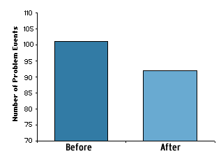
To understand the importance of examining a large number of time periods, consider the following hypothetical example. All the charts that follow are from the same forty period series (shown last in Figure A.4). The response was implemented between periods 19 and 20. Figures A.1 through A.3 show what an evaluator would see if they selected different time periods on either side of the implementation. As you will see, these different views suggest different conclusions.

Fig. A.1. Two-period pre-post design

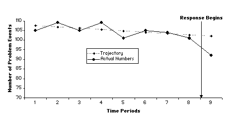
Figure A.2 shows nine time periods–12 through 20 in the series–eight periods before the response, and one after the response. Using more periods provides an opportunity to examine the trend in the problem before the response. The straight line shows this trend (trajectory). Extending the trajectory to one period beyond when response begins allows us to compare what we might expect if the response were not implemented (the trajectory) with the actual problem level. We can plainly see that the problem was trending downward before the response–that is, the response did not cause the entire decline. Nevertheless, it appears that there was a greater drop in the problem after the response than we would have expected due to the trend alone.

Fig. A.2. Nine-period time series design

The periods before the response help establish the trajectory of the problem time series. Here we focused exclusively on the overall trend, but it is also possible to look for seasonal and other recurring fluctuations.

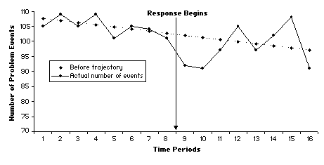
Extending the data to several periods after the response helps us determine the response's stability. Does the response continue to be effective, further reducing the problem? Or does the response wear off, allowing the problem to rebound? Figure A.3 shows an additional seven periods after the response. Based on the pre-response data, the same trend line is used, but it is now projected out eight periods after the response. We see that the problem rebounded and then seemed to oscillate around the trend line. So at best, the response was temporarily helpful.

Fig. A.3. 16-period time series design

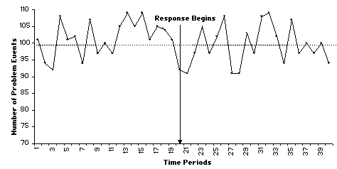
It would be tempting to end the story here, but it is worth examining the entire 40-period series from which the three previous figures were extracted. Figure A.4 shows this series. It turns out that this time series has a flat trajectory. The problem level oscillates around 100 events per period. Further undermining our confidence in the response, we see that there are at least two pre-response periods with declines like those we see after the response. So it appears that what we thought was a decline due to the response may very well be a temporary fluctuation due to normal variations in the problem.

Fig. A.4. 40-period time series design

Unlike real data–with which we are never quite sure of the cause–with this artificial data, we know with absolute certainty that the variations around the 100 events per period are random.† This includes the periods just before and after the response. The example shows that we can easily misinterpret random data fluctuations as meaningful changes. It is worth noting that a significance test to detect randomness in a prepost design might actually suggest that a drop is not due to random changes. This is because randomness affects the entire series, and the pre-post design covers only a small part of the series

† That is because this data series was created by setting a constant level for the problem, and then using a random number generator to provide the fluctuations around that level.